44 excel chart show labels
How to display text labels in the X-axis of scatter chart in Excel? Actually, there is no way that can display text labels in the X-axis of scatter chart in Excel, but we can create a line chart and make it look like a scatter chart. 1. Select the data you use, and click Insert > Insert Line & Area Chart > Line with Markers to select a line chart. See screenshot: 2. charts - Excel, giving data labels to only the top/bottom X% values ... Here is what you can do, in stages: 1) Create a data set next to your original series column with only the values you want labels for (again, this can be formula driven to only select the top / bottom n values). See column D below. 2) Add this data series to the chart and show the data labels. 3) Set the line color to No Line, so that it does ...
EXCEL DO NOT SHOW GRAPH MAP CHART - Microsoft Tech … 08.01.2017 · EXCEL DO NOT SHOW GRAPH MAP CHART. Discussion Options. Subscribe to RSS Feed; Mark Discussion as New; Mark Discussion as Read; Pin this Discussion for Current User; Bookmark; Subscribe; Printer Friendly Page; Mark 777. Occasional Contributor Jan 08 2017 06:56 PM. Mark as New; Bookmark; Subscribe; Mute; Subscribe to RSS Feed; Permalink; …

Excel chart show labels
Excel charts: how to move data labels to legend @Matt_Fischer-Daly . You can't do that, but you can show a data table below the chart instead of data labels: Click anywhere on the chart. On the Design tab of the ribbon (under Chart Tools), in the Chart Layouts group, click Add Chart Element > Data Table > With Legend Keys (or No Legend Keys if you prefer) Display every "n" th data label in graphs - Microsoft Community you can use a free tool created by Rob Bovey, called the XY Chart Labeler. With this tool you can assign a range of cells to be the labels for chart series, instead of the Excel defaults. Using a formula, you can have a text show up in every nth cell and then use that range with the XY Chart Labeler to display as the series label. HOW TO CREATE A BAR CHART WITH LABELS ABOVE BAR IN EXCEL - simplexCT In the chart, right-click the Series "Dummy" Data Labels and then, on the short-cut menu, click Format Data Labels. 15. In the Format Data Labels pane, under Label Options selected, set the Label Position to Inside End. 16. Next, while the labels are still selected, click on Text Options, and then click on the Textbox icon. 17.
Excel chart show labels. Add / Move Data Labels in Charts - Excel & Google Sheets Double Click Chart Select Customize under Chart Editor Select Series 4. Check Data Labels 5. Select which Position to move the data labels in comparison to the bars. Final Graph with Google Sheets After moving the dataset to the center, you can see the final graph has the data labels where we want. Edit titles or data labels in a chart - support.microsoft.com On a chart, click the label that you want to link to a corresponding worksheet cell. On the worksheet, click in the formula bar, and then type an equal sign (=). Select the worksheet cell that contains the data or text that you want to display in your chart. You can also type the reference to the worksheet cell in the formula bar. How to Use Cell Values for Excel Chart Labels - How-To Geek 12.03.2020 · The column chart will appear. We want to add data labels to show the change in value for each product compared to last month. Select the chart, choose the “Chart Elements” option, click the “Data Labels” arrow, and then “More Options.” Uncheck the “Value” box and check the “Value From Cells” box. How to Show Percentage in Pie Chart in Excel? - GeeksforGeeks 29.06.2021 · It can be observed that the pie chart contains the value in the labels but our aim is to show the data labels in terms of percentage. Show percentage in a pie chart: The steps are as follows : Select the pie chart. Right-click on it. A pop-down menu will appear. Click on the Format Data Labels option. The Format Data Labels dialog box will appear.
Excel Charts: Dynamic Label positioning of line series - Xelplus Select your chart and go to the Format tab, click on the drop-down menu at the upper left-hand portion and select Series "Actual". Go to Layout tab, select Data Labels > Right. Right mouse click on the data label displayed on the chart. Select Format Data Labels. Under the Label Options, show the Series Name and untick the Value. How to Add Two Data Labels in Excel Chart (with Easy Steps) You can easily show two parameters in the data label. For instance, you can show the number of units as well as categories in the data label. To do so, Select the data labels. Then right-click your mouse to bring the menu. Format Data Labels side-bar will appear. You will see many options available there. Check Category Name. How to change chart axis labels' font color and size in Excel? Change chart color based on value in Excel Sometimes, when you insert a chart, you may want to show different value ranges as different colors in the chart. For example, when the value range is 0-60, show series color as blue, if 71-80 then show grey, if 81-90 show color as yellow and so on as below screenshot shown. Now this tutorial will ... How to add or move data labels in Excel chart? - ExtendOffice In Excel 2013 or 2016. 1. Click the chart to show the Chart Elements button . 2. Then click the Chart Elements, and check Data Labels, then you can click the arrow to choose an option about the data labels in the sub menu. See screenshot: In Excel 2010 or 2007. 1. click on the chart to show the Layout tab in the Chart Tools group. See screenshot: 2. Then click Data Labels, and select one type of data labels as you need. See screenshot:
Excel Chart Vertical Axis Text Labels • My Online Training Hub 14.04.2015 · To turn on the secondary vertical axis select the chart: Excel 2010: Chart Tools: Layout Tab > Axes > Secondary Vertical Axis > Show default axis. Excel 2013: Chart Tools: Design Tab > Add Chart Element > Axes > Secondary Vertical. Now your chart should look something like this with an axis on every side: How to Add Axis Labels in Excel Charts - Step-by-Step (2022) - Spreadsheeto How to add axis titles 1. Left-click the Excel chart. 2. Click the plus button in the upper right corner of the chart. 3. Click Axis Titles to put a checkmark in the axis title checkbox. This will display axis titles. 4. Click the added axis title text box to write your axis label. How to Add Data Labels to an Excel 2010 Chart - dummies On the Chart Tools Layout tab, click Data Labels→More Data Label Options. The Format Data Labels dialog box appears. You can use the options on the Label Options, Number, Fill, Border Color, Border Styles, Shadow, Glow and Soft Edges, 3-D Format, and Alignment tabs to customize the appearance and position of the data labels. How to Add Total Data Labels to the Excel Stacked Bar Chart 03.04.2013 · For stacked bar charts, Excel 2010 allows you to add data labels only to the individual components of the stacked bar chart. The basic chart function does not allow you to add a total data label that accounts for the sum of the individual components. Fortunately, creating these labels manually is a fairly simply process.
How to Make Charts and Graphs in Excel | Smartsheet
How to Show Percentage in Excel Pie Chart (3 Ways) 03.07.2022 · Display Percentage in Pie Chart by Using Format Data Labels. Another way of showing percentages in a pie chart is to use the Format Data Labels option. We can open the Format Data Labels window in the following two ways. 2.1 Using Chart Elements. To active the Format Data Labels window, follow the simple steps below. Steps:

34 How To Label A Chart In Excel - Label Ideas 2020
Dynamically Label Excel Chart Series Lines - My Online Training Hub Step 1: Duplicate the Series. The first trick here is that we have 2 series for each region; one for the line and one for the label, as you can see in the table below: Select columns B:J and insert a line chart (do not include column A). To modify the axis so the Year and Month labels are nested; right-click the chart > Select Data > Edit the ...
Excel Dashboard Templates Fixing Your Excel Chart When the Multi-Level Category Label Option is ...
How to hide zero data labels in chart in Excel? - ExtendOffice Sometimes, you may add data labels in chart for making the data value more clearly and directly in Excel. But in some cases, there are zero data labels in the chart, and you may want to hide these zero data labels. Here I will tell you a quick way to hide the zero data labels in Excel at once. Hide zero data labels in chart
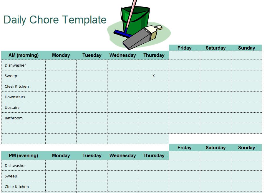
Daily Chore Template
Add or remove data labels in a chart - support.microsoft.com Click the data series or chart. To label one data point, after clicking the series, click that data point. In the upper right corner, next to the chart, click Add Chart Element > Data Labels. To change the location, click the arrow, and choose an option. If you want to show your data label inside a text bubble shape, click Data Callout.

Fixing Your Excel Chart When the Multi-Level Category Label Option is Missing. - Excel Dashboard ...
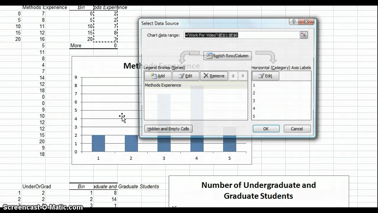
Excel not showing all horizontal axis labels [SOLVED] Re: Excel not showing all horizontal axis labels. I selected the 2nd chart and pulled up the Select Data dialog. I observed: 1) The horizontal category axis data range was row 3 to row 34, just as you indicated. 2) The range for the Mean Temperature series was row 4 to row 34. I assume you intended this to be the same rows as the horizontal ...

Fixing Your Excel Chart When the Multi-Level Category Label Option is Missing. - Excel Dashboard ...
How to show percentage in pie chart in Excel? - ExtendOffice Show percentage in pie chart in Excel. Please do as follows to create a pie chart and show percentage in the pie slices. 1. Select the data you will create a pie chart based on, click Insert > Insert Pie or Doughnut Chart > Pie. See screenshot: 2. Then a pie chart is created. Right click the pie chart and select Add Data Labels from the context ...

Show Trend Arrows in Excel Chart Data Labels
How to Use Cell Values for Excel Chart Labels - How-To Geek Select the chart, choose the "Chart Elements" option, click the "Data Labels" arrow, and then "More Options." Uncheck the "Value" box and check the "Value From Cells" box. Select cells C2:C6 to use for the data label range and then click the "OK" button. The values from these cells are now used for the chart data labels.
Charts in Excel - Easy Excel Tutorial
Unable to see the Label Position in excel chart. 1. Please make sure the options below is checked. 2. The screenshot of Excel version, please go File>Account>Product Information. 3. Does this problem happen on all Excel files with charts? 4. Does this issue happen in Excel files which linked to other files? 5. Does all the labels disappear?

Excel-User.com: Excel Charts - Add totals labels to Stacked Column chart
Data Labels in Excel Pivot Chart (Detailed Analysis) 7 Suitable Examples with Data Labels in Excel Pivot Chart Considering All Factors 1. Adding Data Labels in Pivot Chart 2. Set Cell Values as Data Labels 3. Showing Percentages as Data Labels 4. Changing Appearance of Pivot Chart Labels 5. Changing Background of Data Labels 6. Dynamic Pivot Chart Data Labels with Slicers 7.

How to add or move data labels in Excel chart?
Find, label and highlight a certain data point in Excel scatter graph Here's how: Click on the highlighted data point to select it. Click the Chart Elements button. Select the Data Labels box and choose where to position the label. By default, Excel shows one numeric value for the label, y value in our case. To display both x and y values, right-click the label, click Format Data Labels…, select the X Value and ...
How-to Add Custom Labels that Dynamically Change in Excel Charts - Excel Dashboard Templates
How to Add Labels to Scatterplot Points in Excel - Statology Next, click anywhere on the chart until a green plus (+) sign appears in the top right corner. Then click Data Labels, then click More Options… In the Format Data Labels window that appears on the right of the screen, uncheck the box next to Y Value and check the box next to Value From Cells.

Show Trend Arrows in Excel Chart Data Labels
How to Change Excel Chart Data Labels to Custom Values? 05.05.2010 · We all know that Chart Data Labels help us highlight important data points. When you "add data labels" to a chart series, excel can show either "category" , "series" or "data point values" as data labels. But what if you want to have a data label show a different value that one in chart's source data? Use this tip to do that.

Improve your X Y Scatter Chart with custom data labels
Show Labels Instead of Numbers on the X-axis in Excel Chart Show Labels Instead of Numbers on the X-axis in Excel Chart It is common knowledge that Excel is a great tool for presenting data. When we say that, we do not only mean numerical representation but graphical as well. One of the things that can often bother people and which is not easily achieved is to show labels instead of numbers on the x-axis.
Changing X-Axis Values - YouTube
Excel: How to Create a Bubble Chart with Labels - Statology Step 3: Add Labels. To add labels to the bubble chart, click anywhere on the chart and then click the green plus "+" sign in the top right corner. Then click the arrow next to Data Labels and then click More Options in the dropdown menu: In the panel that appears on the right side of the screen, check the box next to Value From Cells within ...

Creating Pie Chart and Adding/Formatting Data Labels (Excel) - YouTube
Excel Chart Duplicate Labels on X-Axis [SOLVED] Re: Excel Chart Duplicate Labels on X-Axis. If you want to aggregate all the data for Dept 1 for example, then you require a pivot chart rather than a regular chart, or some sort of summary table using formulas. A pivot chart would be the simplest option as it will only need a few mouse clicks to set up.
How to Show Percentages in Stacked Bar and Column Charts in Excel
Excel charts: add title, customize chart axis, legend and data labels Click anywhere within your Excel chart, then click the Chart Elements button and check the Axis Titles box. If you want to display the title only for one axis, either horizontal or vertical, click the arrow next to Axis Titles and clear one of the boxes: Click the axis title box on the chart, and type the text.
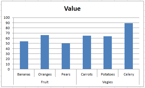
Fixing Your Excel Chart When the Multi-Level Category Label Option is Missing. - Excel Dashboard ...
Add data labels and callouts to charts in Excel 365 - EasyTweaks.com Step #1: After generating the chart in Excel, right-click anywhere within the chart and select Add labels . Note that you can also select the very handy option of Adding data Callouts. Step #2: When you select the "Add Labels" option, all the different portions of the chart will automatically take on the corresponding values in the table ...
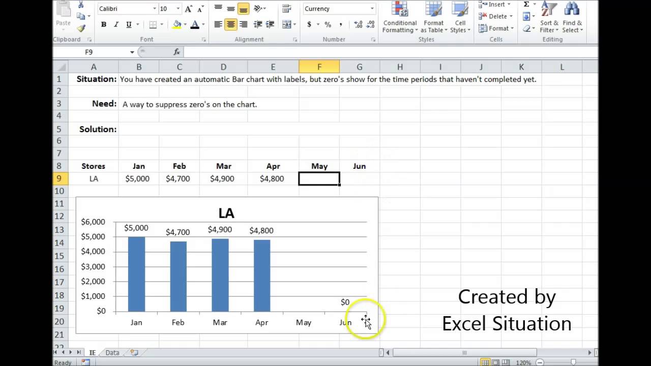
Excel Bar Chart Suppress Zeros - YouTube
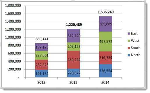
How to Add Labels to Show Totals in Stacked Column Charts in Excel The chart should look like this: 8. In the chart, right-click the "Total" series and then, on the shortcut menu, select Add Data Labels. 9. Next, select the labels and then, in the Format Data Labels pane, under Label Options, set the Label Position to Above. 10. While the labels are still selected set their font to Bold. 11.
Post a Comment for "44 excel chart show labels"